Introduction
This week my boss asked me to gather and produce some LIDAR layers for the island that his family has a cabin on, and I thought it would be a great opportunity to show the workflow for processing compressed LAS point cloud data.
You can download all of the files used in this tutorial by cloning this repository. Included in the repo are the JSON pipelines, the LAS tiles I used, and some scripts to run some of the steps I cover below.
> git clone https://github.com/hadallen/savary-pdal
In this post, I will talk about:
- Software used
- Finding the data
- Processing the point cloud data into raster files with
PDAL - Using
QGISto load and further analyze the raster files - Using
GDALdirectly to analyze the raster files
Interactive Map
Below is an interactive map of the Savary Island LIDAR data, made with Leaflet. The vector & raster data and legend entries are being served from a QGIS Server WMS instance.
Note: I’ve noticed that I had to reload the page to get the map to show sometimes - if you don’t see it below this message then try refreshing
You can switch through the layers by clicking on the layer switcher in the top right corner of the map.
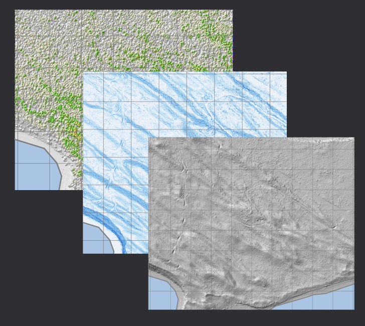
- The Crown Height Model (CHM) shows the difference (in meters) between the Digital Surface Model (DSM) and Digital Terrain Model (DTM). It is overlaid on top of a hillshade made from the DSM for better visualization.
- The DTM Hillshade is a hillshade made from the Digital Terrain Model.
- The Slope Percent shows the slope (rise/run) of the terrain in percent. For example, a slope of 50% means that a horizontal distance of 50 meters would result in a vertical rise of 25 meters.
Software used
- PDAL 2.4.2 - The main software used to process the LAZ point clouds:
PDAL is Point Data Abstraction Library. It is a C/C++ open source library and applications for translating and processing point cloud data. 1
- GDAL 3.5.1 - A extremely useful C/C++ library and set of command line tools for reading and writing raster and vector data.
GDAL is a translator library for raster and vector geospatial data formats that is released under an MIT style Open Source License by the Open Source Geospatial Foundation. 2
- QGIS 3.26.1-Buenos Aires - Used to view the resulting raster files, and can be used to simplify the use of gdal algorithms.
QGIS is a user friendly Open Source Geographic Information System (GIS) licensed under the GNU General Public License. QGIS is an official project of the Open Source Geospatial Foundation (OSGeo). It runs on Linux, Unix, Mac OSX, Windows and Android and supports numerous vector, raster, and database formats and functionalities. 3
Gathering the data
Getting your hands on point cloud data can be pretty hit or miss. You may be able to find an online resource, like LidarBC. This is a service that allows you to browse & download tiles from the province of British Columbia’s collection of LIDAR point cloud (some derivative raster data is also available).
There may be similar services for your province, county, state, city, or country. Some countries have regularly updated country-wide datasets that are freely accessible. Some countries have more limited access to data, but you may be able to find some data for your region of interest.
Check out this article or do a quick internet search for “(Your area of interest) LIDAR data” to see if you can track down open data for the area you are interested in.
Be sure to check the licensing information for the data you download, and follow it accordingly.
Once I found the tiles that I was interested in, I downloaded each of them and put them in a folder savary-pdal/tiles. These will be read by PDAL and processed into raster data.
Processing Workflow
Setting up the pipelines
Although you can use PDAL command line options to provide all of the information needed to process the data, I find it a lot simpler to use PDAL’s pipeline option. This allows you to save the configuration and use it for multiple datasets, or share it with others.
Pipelines allow you to layout your workflow in a way that is easy to understand and share. Basically, in the pipeline file, you define the steps that will be executed in order. You can also define the input and output files, and the parameters that will be used for reading and writing the files.
Below is an example pipeline from PDAL’s documentation. It is a simple workflow that reads input.las using readers.las, applies the filters.crop filter to extract the points within the specified bounds in the follow format: "([xmin, xmax], [ymin, ymax])",and then writes the file to output.bpf using writers.bpf.
| |
Refer to PDAL’s pipeline documentation for more information.
Creating the Digital Surface Model (DSM) pipeline
To create a digital surface model from the point clouds, we are only interested in the points that reflected off the top of the trees, buildings, and other objects - not the ones that penetrated the canopy and bounced off the ground.
Although I don’t in this example, you could potentially use the filters.outliers filter (like we do in the DTM Pipeline to remove the points that may be “noise” or “static”.
Pipeline example: generate-dsm.json
| |
In the generate-dsm.json pipeline above, you can see:
readers.lasis used to set the input file type. If you are only using a single file, you can use thefilenameoption here.filters.reprojectionis used to reproject the data from one CRS to another (EPSG:6653 to EPSG:3157). CRS’s are used to define the coordinate system of the data and can be extremely confusing & a common source of errors. Make sure you know the CRS of the data you are working with and that all data is reprojected to the same CRS, if needed.filters.rangeis used to isolate ONLY the 1st return points. This filters only the 1st return points, which are the ones that reflected off the top of the trees, buildings, and other objects. Only these filtered points will be passed onto the next stage.writers.gdalis used to write the set the options for the output file."gdaldriver":"GTiff": the gdal driver is set toGTifffor a GeoTIFF. I suggest translating it to a Cloud Optimized GeoTIFF (COG) as an additional step after analysis is finished, as it is internally tiled and has better compression."resolution": 0.5: the resolution of the is set to 0.5m, which is very detailed. This is the height and width of each pixel in the output raster. The resolution can greatly affect the size of the output file, so for larger datasets, you may need to use a lower resolution.
You may notice that although I specify the readers and writers, I do not specify the filename. This is because we need to add an additional step to analyze our tiled LAZ files. If I was running a single file through the pipeline, I could specify the filenames in pipeline or use the following command:
pdal pipeline ./generate-dsm.json \
    --readers.las.filename=tiles/bc_092f096_2_3_2_xyes_8_utm10_2019.laz \
    --writers.gdal.filename=out/dsm/dsm_bc_092f096_2_3_2_xyes_8_utm10_2019.tif
Creating the Digital Terrain Model (DTM) pipeline
Now that our pipeline for the Digital Surface Model (DSM) is ready, we can create the pipeline for the Digital Terrain Model (DTM).
This takes a bit more work, because we need to do some classification and further filtering of our data to clean it up and extract the ground information.
Pipeline example: generate-dtm.json
| |
You will notice that the readers.las , filters.reprojection, and writers.gdal stages are the same as the DSM pipeline. However, there are a few more stages added to the pipeline.
Cleaning up the data (denoise, remove outliers, etc.)
Point cloud data can often contain points that will throw off your analysis. There are a few easy filters that can be used to clean up data, removing this “noise” that results in a smoother terrain surface.
First, the
filters.assignstage is used to clear the classification values. Your data may already be classified, but you may not know the accuracy of the classification or you may need to do it yourself with specific options.Next is the
filters.elmstage, which is the Extended Local Minimum (ELM) filter. It classifies low points in the data as classification 7. Similarly, thefilters.outlierstage is used to remove outliers. This is a filter that removes points that are too far from the average of the points in their neighborhood, and marks them as classification 7 as well. These will be ignored in the next step.
Classifying the ground points
Now that we have cleaned up the point cloud data, we can begin to classify the points as ground or non-ground using the filters.smrf (Simple Morphological Filter). This filter assigns ground points to the classification value of 2, which we will filter out using filters.range, which will be passed to writers.gdal to write the output file.
The options for filters.smrf can be found on the documentation and tweaked to better suit your needs.
Similar to the DSM, if I was running a single file through the pipeline, I could specify the filenames in pipeline or use the following command:
pdal pipeline ./generate-dtm.json \
    --readers.las.filename=tiles/bc_092f096_2_3_2_xyes_8_utm10_2019.laz \
    --writers.gdal.filename=out/dtm/dtm_bc_092f096_2_3_2_xyes_8_utm10_2019.tif
Running batch pipelines using parallel
PDAL has a great write-up on batch processing in the Workshop section. I will go through the process I used, using ls and parallel in bash or zsh, but if you are on Windows, you can follow the instructions in the write-up.
Creating the list of files with ls
To begin, I needed an ls command that will list ONLY the tiles that I was interested in processing.
Since I have all of my tiles in a single directory, I can use the ls command from inside the tiles directory to list all of the files inside.
> cd tiles         # modify this to the directory where your tiles are

> ls               # lists all the files in the current directory
bc_092f096_2_3_2_xyes_8_utm10_2019.laz  bc_092f096_2_4_4_xyes_8_utm10_2019.laz
bc_092f096_2_3_4_xyes_8_utm10_2019.laz  bc_092f097_1_3_1_xyes_8_utm10_2019.laz
bc_092f096_2_4_1_xyes_8_utm10_2019.laz  bc_092f097_1_3_3_xyes_8_utm10_2019.laz
bc_092f096_2_4_2_xyes_8_utm10_2019.laz  bc_092f097_1_3_4_xyes_8_utm10_2019.laz
bc_092f096_2_4_3_xyes_8_utm10_2019.laz  bc_092f097_3_1_2_xyes_8_utm10_2019.laz
If I had many tiles in that directory but I only wanted to process some of them, I just could use the ls bc_*.laz command to list all of the files that match bc_*.laz. Adjust this to your dataset as needed.
> cd tiles         # modify this to the directory where your tiles are

> ls bc_*.laz      # lists all files that match the pattern 'bc_*.laz'
bc_092f096_2_3_2_xyes_8_utm10_2019.laz  bc_092f096_2_4_4_xyes_8_utm10_2019.laz
bc_092f096_2_3_4_xyes_8_utm10_2019.laz  bc_092f097_1_3_1_xyes_8_utm10_2019.laz
bc_092f096_2_4_1_xyes_8_utm10_2019.laz  bc_092f097_1_3_3_xyes_8_utm10_2019.laz
bc_092f096_2_4_2_xyes_8_utm10_2019.laz  bc_092f097_1_3_4_xyes_8_utm10_2019.laz
bc_092f096_2_4_3_xyes_8_utm10_2019.laz  bc_092f097_3_1_2_xyes_8_utm10_2019.laz
Running the list of files through parallel
Now that I have the list of files, I can use parallel to run each pipeline on each tile:
> cd tiles         # modify this to the directory where your tiles are

> ls bc_092f09*.laz | parallel -I{} \
    pdal pipeline ../generate_dsm.json \ # adjust this if needed
    --readers.las.filename={} \
    --writers.gdal.filename=../out/dsm/dsm_{/.}.tif

> ls bc_092f09*.laz | parallel -I{} \
    pdal pipeline ../generate_dtm.json \ # adjust this if needed
    --readers.las.filename={} \
    --writers.gdal.filename=../out/dtm/dtm_{/.}.tif
In this command, each file from the list is passed to parallel as an argument. The {} is a placeholder for the file name. The {/.} is a placeholder for the file name without the extension.
Since the filename option is not set in our pipeline, we have to define it in each command for the reader and writer:
readers.las.filenameis set to{}, which will pass the entire filename- e.g.
bc_092f096_2_3_2_xyes_8_utm10_2019.lazwill be passed toPDAL
- e.g.
writers.gdal.filenameis set to..out/dsm/dsm_{/.}.tif- Make sure that the output directory exists
- e.g.
../out/dsm/dsm_bc_092f096_2_3_2_xyes_8_utm10_2019.tifwill be passed toPDAL
Checking the output
Each command will take an increasing amount of time based on the density of the point cloud, the size & number of tiles, and the resolution option in the writers.gdal stage of your pipeline.
Once each batch pipeline is complete, check the folder that you set as the output directory.
> cd ..

> ls out/dsm
dsm_bc_092f096_2_3_2_xyes_8_utm10_2019.tif  dsm_bc_092f096_2_4_4_xyes_8_utm10_2019.tif
dsm_bc_092f096_2_3_4_xyes_8_utm10_2019.tif  dsm_bc_092f097_1_3_1_xyes_8_utm10_2019.tif
dsm_bc_092f096_2_4_1_xyes_8_utm10_2019.tif  dsm_bc_092f097_1_3_3_xyes_8_utm10_2019.tif
dsm_bc_092f096_2_4_2_xyes_8_utm10_2019.tif  dsm_bc_092f097_1_3_4_xyes_8_utm10_2019.tif
dsm_bc_092f096_2_4_3_xyes_8_utm10_2019.tif  dsm_bc_092f097_3_1_2_xyes_8_utm10_2019.tif

> ls out/dtm
dtm_bc_092f096_2_3_2_xyes_8_utm10_2019.tif  dtm_bc_092f096_2_4_4_xyes_8_utm10_2019.tif
dtm_bc_092f096_2_3_4_xyes_8_utm10_2019.tif  dtm_bc_092f097_1_3_1_xyes_8_utm10_2019.tif
dtm_bc_092f096_2_4_1_xyes_8_utm10_2019.tif  dtm_bc_092f097_1_3_3_xyes_8_utm10_2019.tif
dtm_bc_092f096_2_4_2_xyes_8_utm10_2019.tif  dtm_bc_092f097_1_3_4_xyes_8_utm10_2019.tif
dtm_bc_092f096_2_4_3_xyes_8_utm10_2019.tif  dtm_bc_092f097_3_1_2_xyes_8_utm10_2019.tif
Now that we have our DSM and DTM, we will view, organize, and further process them using QGIS and GDAL.
Working with the GeoTIFF Rasters in QGIS and GDAL
Open up QGIS and create a new project. Set the CRS of your project to the same CRS that you reprojected your data into in the pipeline, in my case it is EPSG:3157.
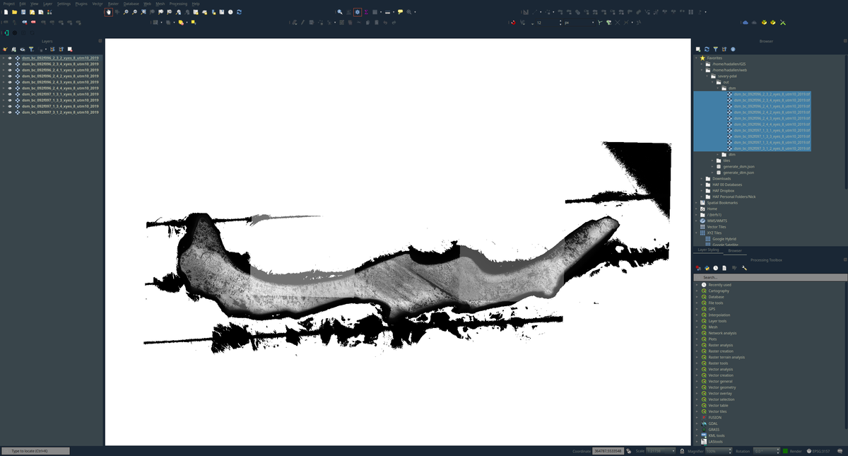
The QGIS window is shown above, with all of the DSM tiles loaded into a new project.
There are several ways to add the raster files to your project. You can drag in one or all of the TIFF files from your file explorer into QGIS, or use the browser panel to navigate to the folder that you set as the output directory, then drag them into the canvas area. You can also use the Data Source Manager to add any type of data.
Creating a virtual raster layer
After you’ve loaded all the raster tiles, you can create a virtual raster layer by going to:Raster > Miscellaneous > Build Virtal Raster...
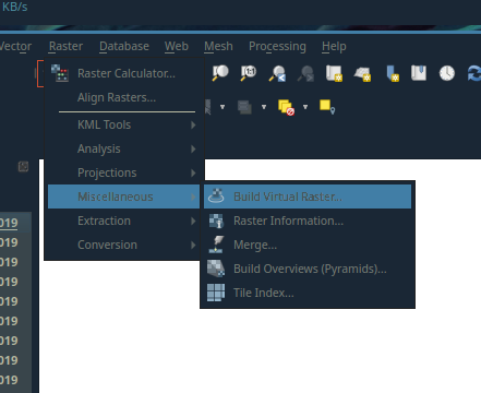
Location of the Build Virtual Raster... tool
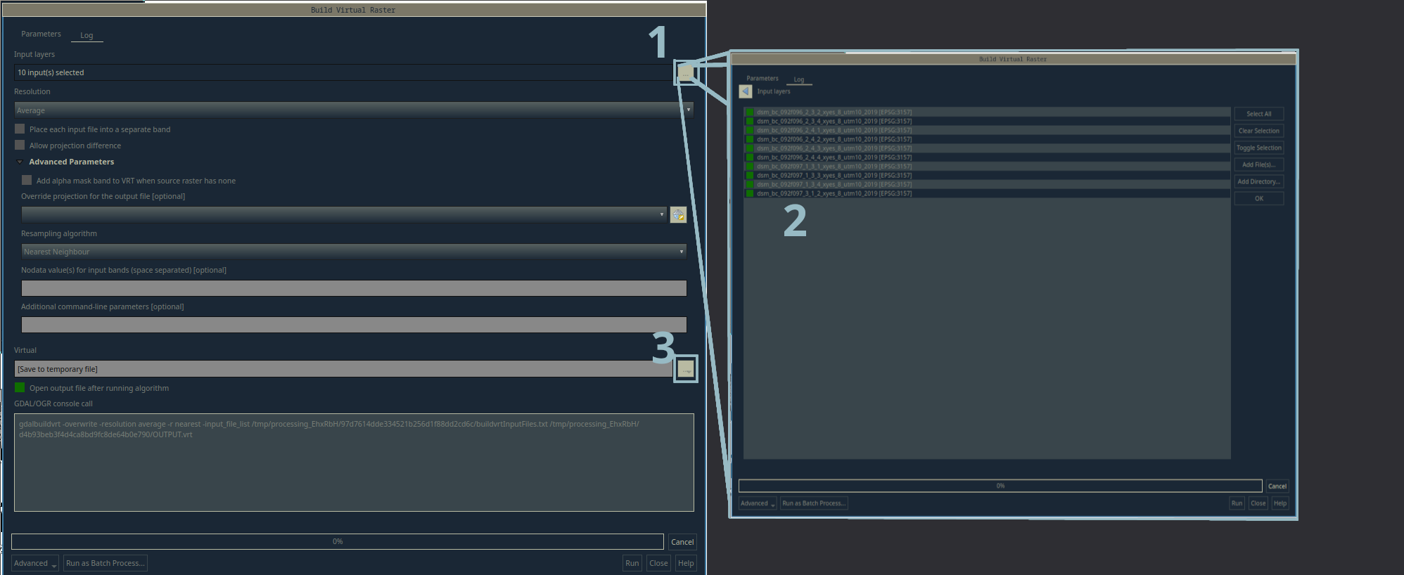
The Build Virtual Raster tool and the layer selection window
- Click the
...button and add all of the tiles of one set (i.e. the 10 individualdsm_bc_..._x_y_x.tiftiles) to the layer selection window. - You can use this window to add layers that are already in the project, or you can add an entire directory using the buttons on the right hand side.
- You can choose a location to save the virtual raster by clicking the
...button and selecting a location. If you leave it blank, it will be added to the project as a temporary layer. - Click the
OKbutton and your virtual raster will be created.
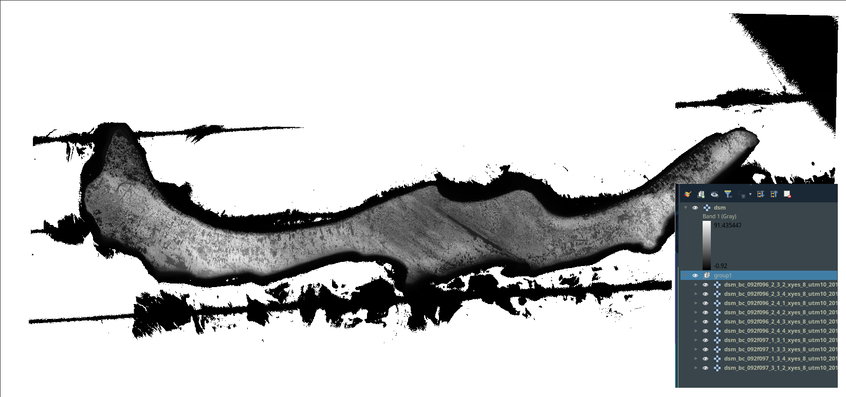
Once the Build Virtual Raster tool runs, you will see the entire mosaic combined into one continuous layer. In the foreground, you can see that layers panel shows the dsm virtual raster at the top, and a group of the tiles below.
If you don’t see the virtual raster on your canvas, you may have to rearrange the layers in the layer panel.
Do this for both the DSM and DTM rasters tile sets and take a look at each of them. Style them if you’d like - this won’t be covered in this article.
If you look at the bottom of the Build Virtual Raster tool, you can see the command that is run to fill in the gaps. A similar command can be seen at the bottom of each raster tool we cover in this article.
These are the GDAL command line tools that QGIS is running, and you can use them yourself to run these tools from the command line. I will include them with each analysis step in this article.
gdalbuildvrt command
# build virtual raster commands
> gdalbuildvrt -overwrite -resolution average -r nearest \
    -input_file_list /path/to/DSM_Tile_List \
    /home/hadallen/web/savary-pdal/out/dsm/dsm.vrt

> gdalbuildvrt -overwrite -resolution average -r nearest \
    -input_file_list /path/to/DTM_Tile_List \
    /home/hadallen/web/savary-pdal/out/dtm/dtm.vrt
Filling gaps in the raster
If you look closely, you can see that there are areas in each raster where there are large gaps of no data. One solution for this is the run the Raster > Analysis > Fill nodata... tool.

Fill Nodata tool location in QGIS
Use the Fill nodata tool for each virtual raster layer. Take a look at the new layer and compare it to the original. You can see that most of the gaps have been filled in, but some remain. If needed, you can increase the Maximum distance (in pixels) to search out for values to interpolate option to fill in more gaps.
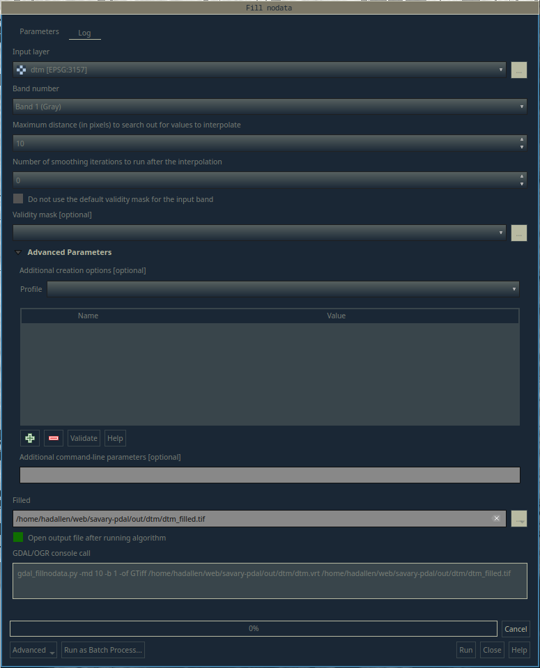
Fill Nodata tool in QGIS
gdal_fillnodata.py command
# fill nodata commands
> gdal_fillnodata.py -md 10 -b 1 -of GTiff \
    /home/hadallen/web/savary-pdal/out/dtm/dsm.vrt \
    /home/hadallen/web/savary-pdal/out/finals/dsm_filled.tif

> gdal_fillnodata.py -md 10 -b 1 -of GTiff \
    /home/hadallen/web/savary-pdal/out/dtm/dtm.vrt \
    /home/hadallen/web/savary-pdal/out/finals/dtm_filled.tif
Generating Crown Height Model (CHM) using gdal_calc.py
Now that we have filled in the gaps in the rasters, we can use the gdal_calc.py command to generate the CHM.
> gdal_calc.py -A out/finals/dtm_filled.tif -B out/finals/dsm_filled.tif \
    --calc="B-A" --outfile out/finals/chm.tif --extent intersect
Generating Hillshade and Slope rasters
In the same menu in QGIS, you can go to Raster > Analyis > Slope or Hillshade to produce the respective raster layers.
In the Slope tool, you must be sure to select the Slope expressed at percent instead of degrees option in order to get the slope in Percent (rise/run) rather than in degrees.

Slope tool in QGIS
Run the Hillshade tool on both the DSM-filled.tif and the DTM-filled.tif rasters. We will use the DSM hillshade with the Crown Height Model for better visualization. The DTM Hillshade can be used to view the topography of the DTM.

Hillshade tool in QGIS
gdaldem command for hillshade and slope
# hillshade commands
> gdaldem hillshade /home/hadallen/web/savary-pdal/out/finals/dsm_filled.tif \
    /home/hadallen/web/savary-pdal/out/finals/dsm_hillshade.tif \
    -of GTiff -b 1 -z 1.0 -s 1.0 -az 315.0 -alt 45.0

> gdaldem hillshade /home/hadallen/web/savary-pdal/out/finals/dtm_filled.tif \
    /home/hadallen/web/savary-pdal/out/finals/dtm_hillshade.tif \
    -of GTiff -b 1 -z 1.0 -s 1.0 -az 315.0 -alt 45.0


# slope command
> gdaldem slope /home/hadallen/web/savary-pdal/out/finals/dtm_filled.tif  \
    /home/hadallen/web/savary-pdal/out/finals/slope.tif \
    -of GTiff -b 1 -s 1.0 -p
Additional Resources
Clipping the rasters
Another tool that you may want to use is the gdalwarp command line tool. I won’t cover this here, but you use this to clean up the edges of the raster files.
gdalwarp -of GTiff -cutline ../savary_polygon.shp -cl savory_polygon \
  -crop_to_cutline out/dtm/dtm-filled.tif out/dtm/dtm-filled-cropped.tif
Others Sources
- PDAL has a great collection of documentation, particularly useful were the Workshop section & Batch Processing page.
- GDAL is a great tool for working with rasters, and many tutorials, and the GIS Stack Exchange is a great collection of GDAL questions.
- QGIS has an excellent set of documentation for working with raster and vector data, WMS/WFS web services, and much more. You can work with LAZ files in QGIS, however I find it to be a bit cumbersome to use for large datasets and more efficient to work in the command line.
- https://www.simonplanzer.com/articles/lidar-chm/ this was an extremely valuable resource when I was first working with the data.
- https://gisgeography.com/top-6-free-lidar-data-sources/